Affiliate links on Android Authority may earn us a commission. Learn more.
How to freeze cells in Excel
If you have ever used Excel to review a large database, you know how useful it is to be able to freeze cells, such as the top row or the first column. It’s so handy because these two places are where your headings are. Freezing the top row or first column lets you keep your headings visible as you scroll through rows and columns of data. It’s easy to do, but with Excel’s rich feature set, the control for it might be a little hard to find. We’ll lead you right to it.
Read more: How to add cells in Excel
QUICK ANSWER
With Excel open, go to View > Freeze Panes. Choose Freeze Top Row to keep row 1 visible no matter how far down you scroll.
JUMP TO KEY SECTIONS
How to freeze the top row in Excel
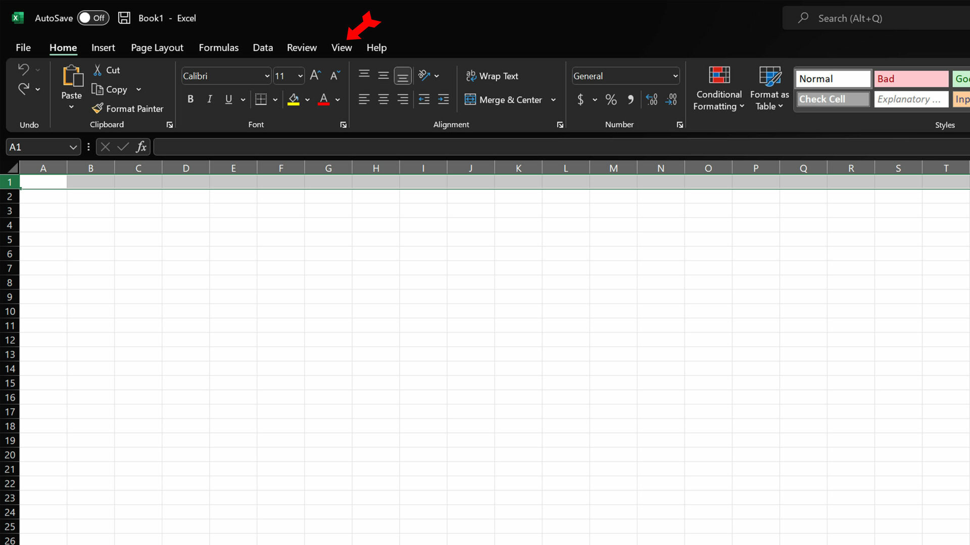
With Excel open, click on the View menu at the top of the page.
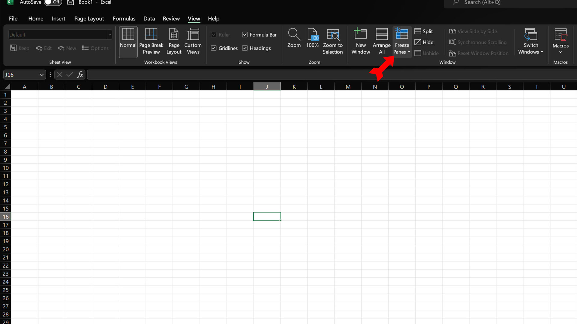
In the View menu, click on the Freeze Panes button.
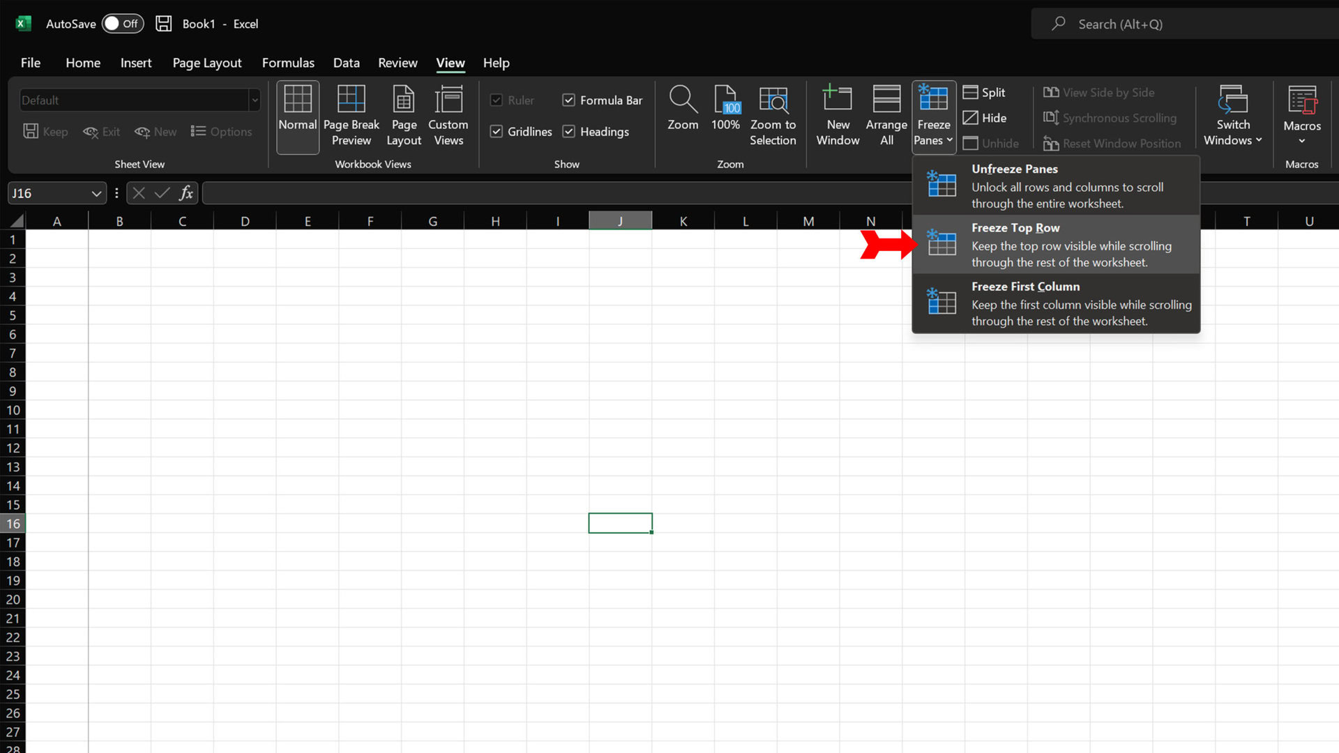
From the menu that drops down, select Freeze Top Row.
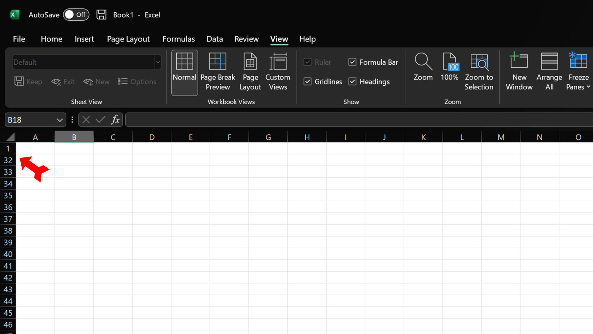
As you can see, when we scroll down through the worksheet, Row 1 is still visible.
How to freeze the first column in an Excel worksheet
Follow the instructions above but, when you click on the Freeze Panes button, select Freeze First Column.
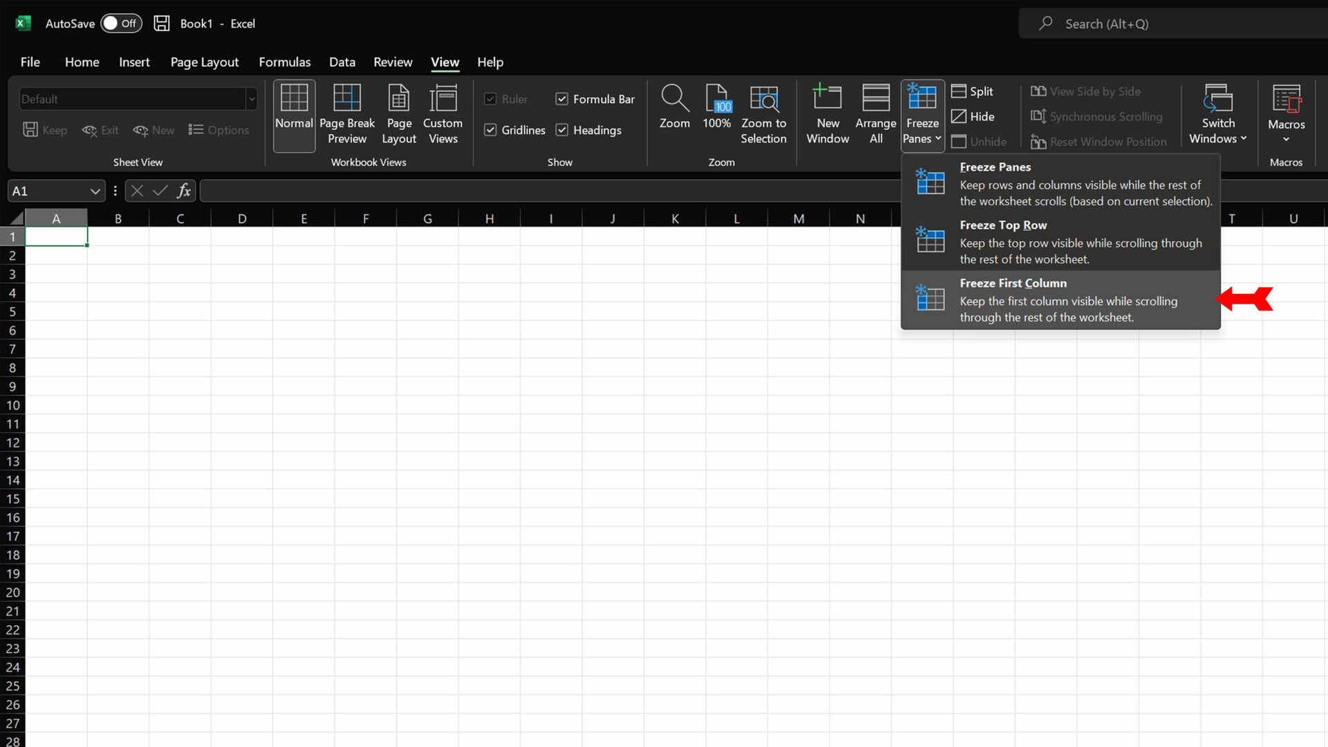
The first column will now stay in view as we scroll to the right.
How to freeze rows and columns at the same time
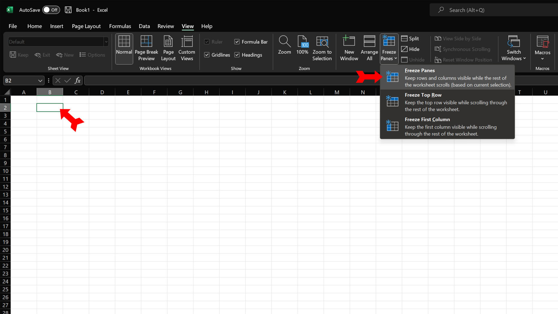
If you have headers both along the top and down the left side of your worksheet, it makes sense to freeze them both. You can do this by choosing the third choice inside the Freeze Panes button, Freeze Panes.
This is a very flexible command, which will let you freeze as many panes (cells), vertically or horizontally, as you want. How many will be frozen depends on which cells you have selected at the time you freeze the panes. Specifically, to freeze just the top row and the leftmost column, select cell B2.
Now activate the Freeze Panes command. Excel will freeze every column to the left of B2 and every row above B2. In other words, Row 1 and Column A are now frozen. You can now scroll through any size worksheet, horizontally or vertically, without losing sight of your headings.
FAQs
The cell is not wide enough to display the whole text. Grab the right border of the cell and move it rightward to make the column wider.
Yes, there are free online versions of all the Office apps available at www.office.com.
Go to the View ribbon and, under the Show section, check the box labeled Headings. Your row numbers and column letters will return.
Thank you for being part of our community. Read our Comment Policy before posting.